- Markov Chain Monte Carlo methods
- Metropolis Hastings
- Gibbs
- convergence / representativeness
- trace plots
- R hat
- efficiency
- autocorrelation
- effective sample size
key notions
recap
Bayes rule for data analysis:
\[\underbrace{P(\theta \, | \, D)}_{posterior} \propto \underbrace{P(\theta)}_{prior} \times \underbrace{P(D \, | \, \theta)}_{likelihood}\]
normalizing constant:
\[ \int P(\theta') \times P(D \mid \theta') \, \text{d}\theta' = P(D) \]
easy to solve only if:
- \(\theta\) is a single discrete variable with reasonably sized domain
- \(P(\theta)\) is conjugate prior for the likelihood function \(P(D \mid \theta)\)
- we are very lucky
approximation by sampling
example: normal distribution
# get density values and samples
xVec = seq(-4, 4, length.out = 10000)
xDense = dnorm(xVec, mean = 0, sd = 1) # density of a standard normal
xSamples = rnorm(10000, mean = 0, sd = 1) # 10000 samples from a standard normal
# plot actual densities and estimated densities from samples
plotData = data.frame(xSamples = xSamples) # put data in data frame for plotting
myPlot = ggplot(data = plotData, aes(x = xSamples)) + # prepare plot
geom_density() + # density estimates
geom_line(x = xVec, y = xDense, color = "blue") + # actual densities
xlab("x") + ylab("(estimated) probability") + # axis labels
theme(plot.background=element_blank()) # transparent background
show(myPlot)
notation
- \(X = (X_1,\dots,X_k)\) is a vector of random variables
- think \(\theta\), but here more generally any \(X\)
- \(x\) is a realization (or particular value) of \(X\)
- distribution of \(X\) is \(P\), to be written as \(X \sim P\)
examples:
- \(X \sim N(\mu,\sigma)\)
- read: "\(X\) is normally distributed with mean \(\mu\) and SD \(\sigma\)"
- \(\theta \sim \text{beta}(a,b)\)
- read: "\(\theta\) comes from a beta distribution with shape \(a\) and \(b\)"
why simulate?
problem:
- assume that \(X \sim P\) and that \(P\) is "unwieldy"
- we'd like to know: \(f(X)\)
- e.g., mean/median/sd of \(X\), 95% HDI, \(\dots\)
- or, marginalized distribution over \(X_i\)
dummy
solution:
-
Monte Carlo simulation
- draw samples \(S\) from \(P\)
- calculate \(f(S)\)
- for many \(f\), \(f(S)\) will approximate \(f(X)\) if \(S\) is "representative" of \(P\)
Markov chains
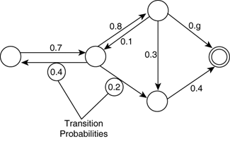
Markov chain
intuition
- a sequence of elements from \(X\), \(x_0, x_1, \dots, x_n\) such that every \(x_{i+1}\) depends only on its predecessor \(x_i\)
- think: probabilistic finite state machine

Markov property
\[P(X_{n+1} = x_{n+1} \mid X_0 = x_0, \dots, X_n = x_n) = P(X_{n+1} = x_n \mid X_n = x_n)\]
Markov Chain Monte Carlo methods
get sequence of samples from \(X \sim P\) s.t. every sample depends on its predecessor, such that:
- the stationary distribution of the chain is \(P\)
- ideally, only few steps are necessary to get representative samples of \(P\)
dummy
- bad: non-independence -> autocorrelation
- good: no need to bother with normalizing constant
Metropolis Hastings
island hopping

- set of islands \(X = \{x_1, x_2, \dots x_n\}\)
- goal: hop around & visit every island \(x_i\) proportional to its population \(P(x_i)\)
- think: "samples" from \(X \sim P\)
- problem: island hopper can remember at most 2 islands' population
- think: we don't know the normalizing constant
Metropolis Hastings
- let \(f(x) = \alpha P(x)\) (e.g., unnormalized posterior)
- start at random \(x^0\), define probability \(P_\text{trans}(x^i \rightarrow x^{i+1})\) of going from \(x^{i}\) to \(x^{i+1}\)
- proposal \(P_\text{prpsl}(x^{i+1} \mid x^i)\): prob. of considering jump to \(x^{i+1}\) from \(x^{i}\)
- acceptance \(P_\text{accpt}(x^{i+1} \mid x^i)\): prob of making jump when \(x^{i+1}\) is proposed \[P_\text{accpt}(x^{i+1} \mid x^i) = \text{min} \left (1, \frac{f(x^{i+1})}{f(x^{i})} \frac{P_\text{prpsl}(x^{i} \mid x^{i+1})}{P_\text{prpsl}(x^{i+1} \mid x^i)} \right)\]
- transition \(P_\text{trans}(x^i \rightarrow x^{i+1}) = P_\text{prpsl}(x^{i+1} \mid x^i) \times P_\text{accpt}(x^{i+1} \mid x^i)\)
7-island hopping
7-island hopping, cont.
properties MH
- motto: always up, down with probability \(\frac{f(x^{i+1})}{f(x^{i})}\)
- ratio \(\frac{f(x^{i+1})}{f(x^{i})}\) means that we can forget about normalizing constant
- \(P_\text{trans}(x^i \rightarrow x^{i+1})\) defines transition matrix -> Markov chain analysis!
- for suitable proposal distributions:
- stationary distribution exists (first left-hand eigenvector)
- every initial condition converges to stationary distribution
- stationary distribution is \(P\)
influence of proposal distribution
Gibbs sampling
Gibbs sampling: introduction
- Metropolis is a very general and versatile algorithm
- however in specific situations, other algorithms may be better applicable
- for example, if \(X=(X_1,\dots,X_k)\) is a vector of random variables and \(P(x)\) is a multidimensional distribution
- in such cases, the Gibbs sampler may be helpful
- basic idea: split the multidimensional problem into a series of simpler problems of lower dimensionality
Gibbs sampling: main idea
- assume \(X=(X_1,X_2,X_3)\) and \(p(x)=P(x_1,x_2,x_3)\)
- start with \(x^0=(x_1^0,x_2^0,x_3^0)\)
- at iteration \(t\) of the Gibbs sampler, we have \(x^{i-1}\) and need to generate \(x^{i}\)
- \(x_1^{i} \sim P(x_1|x_2^{i-1},x_3^{i-1})\)
- \(x_2^{i} \sim P(x_2|x_1^{i},x_3^{i-1})\)
- \(x_3^{i} \sim P(x_3|x_1^{i},x_2^{i})\)
- for a large \(n\), \(x^n\) will be a sample from \(P(x)\)
- \(x^n_k\) will be a sample from \(P(x_k)\) (marginal distribution)
example: 2 coin flips
example: Gibbs jumps
example: Gibbs for 2 coin flips
example: MH for 2 coin flips
summary
- Gibbs sampling can be more efficient than MH
- Gibbs needs samples from conditional posterior distribution
- MH is more generally applicable
- preformance of MH depends on proposal distribution
clever software helps determine when/how to do Gibbs and how to tune MH's proposal function (next class)
assessing sample chains
problem statements
convergence/representativeness
- we have samples from MCMC, ideally several chains
- in the limit, samples must be representative of \(P\)
- how do we know that our meagre finite samples are representative?
efficiency
- ideally, we'd like the shortest samples that are representative
- how do we measure that we have "enough" samples?
packages to compare MCMC chains
require('coda')
require('ggmcmc')

coda and ggmcmc basically do the same thing, but they differ in, say, aesthetics
example MCMC data
out = MH(f, 60000,2,10000) # this is the output of the program of Ex 4 in HW 2
# its an MCMC-list from 'coda' package: i.e., a list
# of MCMC-objects
show(summary(out))
## ## Iterations = 1:50000 ## Thinning interval = 1 ## Number of chains = 2 ## Sample size per chain = 50000 ## ## 1. Empirical mean and standard deviation for each variable, ## plus standard error of the mean: ## ## Mean SD Naive SE Time-series SE ## mu 0.004904 0.07475 0.0002364 0.0012889 ## sigma 1.051322 0.05314 0.0001680 0.0008058 ## ## 2. Quantiles for each variable: ## ## 2.5% 25% 50% 75% 97.5% ## mu -0.1484 -0.0424 0.006156 0.0562 0.1471 ## sigma 0.9537 1.0136 1.050294 1.0867 1.1619
example MCMC data
out2 = ggs(out) # cast the same information into a format that 'ggmcmc' uses show(head(out2)) # this is now a data.frame
## Source: local data frame [6 x 4] ## ## Iteration Chain Parameter value ## (int) (int) (fctr) (dbl) ## 1 1 1 mu -0.01714470 ## 2 2 1 mu -0.09520337 ## 3 3 1 mu -0.09520337 ## 4 4 1 mu -0.09520337 ## 5 5 1 mu -0.09520337 ## 6 6 1 mu -0.09520337
trace plots in 'coda'
plot(out)
trace plots in 'ggmcmc'
ggs_traceplot(out2)
visual inspection of convergence
EJ Wagenmakers:
- trace plots from multiple chains should look like:
- caterpillars madly in love with each other
examining sample chains: beginning
examining sample chains: rest
R hat
\(\hat{R}\)-statistics,
- a.k.a.:
- Gelman-Rubin statistics
- shrink factor
- potential scale reduction factor
- idea:
- compare variance within a chain to variance between chains
- in practice:
- use software to compute it
- aim for \(\hat{R} \le 1.1\) for all continuous variables
R hat in 'coda'
gelman.diag(out)
## Potential scale reduction factors: ## ## Point est. Upper C.I. ## mu 1 1.00 ## sigma 1 1.01 ## ## Multivariate psrf ## ## 1
R hat in 'ggmcmc'
ggs_Rhat(out2)
autocorrelation
autocorrelation in 'coda'
autocorr.plot(out)
autocorrelation in 'ggmcmc'
ggs_autocorrelation(out2)
effective sample size
- intuition:
- how many samples are "efficient, actual samples" if we strip off autocorrelation
- definition:
\[\text{ESS} = \frac{N}{ 1 + 2 \sum_{k=1}^{\infty} ACF(k)}\]
effective sample size in 'coda'
effectiveSize(out)
## mu sigma ## 3365.707 4355.494
next time
homework for next week
- read Kruschke Chapter 8 in preparation
- install JAGS
- hand in homework 2